Overview

Correlation, the previous topic, is very closely related to regression.

Correlation Correlation is a statistical technique that is used to measure and describe the strength of the relationship between two (or more) variables. Regression Regression is a statistical technique that is used to measure and describe the function relating two (or more) variables.

Recall that we presented some examples that used variables about characteristics of automobiles. We showed the relationship between two of these variables, the Weight (in Tons) of automobiles and the Horsepower of their engines.

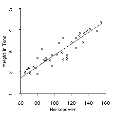
Weight and Horsepower Correlation: The relationship between Weight and Horsepower is strong, linear, and positive, though not perfect. Pearson R = +.92 Regression: The straight line is the regression line. It is the best straight line in describing the relationship between weight and horsepower. The line has the equation: Wt = .37 + .02*Hpwr

Correlation:

Correlation tells us about the strength (and shape) of the relationship between these two variables. The Pearson correlation for weight and horsepower is +0.92. This value tells us that there is a very strong linear relationship between them. In fact, the square of the correlation, which is 0.83, tells us that 83% of their variance is shared between them.

Regression:

Regression tells us about the nature of the function relating the two variables. For linear regression, which is what we consider here, regression fits a straight line to the data so that the line best describes their relationship. The regression line, as the line is called, has been added to the scatterplot above.

Regression Analysis

Regression analysis fits a straight line to the relationship between the two variables. The line that is fit to the relationship has certain properties.

The Regression Line

• is as close as possible, in a specific average least squares sense, to all of the points.

• identifies the "central tendency" of the relationship between the two variables, just as the mean identifies the "central tendency" of a single variable.

• provides a simplified description --- a model --- of the relationship between the two variables.

• gives us a way to predict values for the response variable from values of the predictor variable.

Equation for a Straight Line


Any straight line is described by the linear equation for two variables X and Y. The general equation for a straight line is:

This equation shows that any straight line can be described by just two values. These are its:
1. Intercept: Intercept is denoted by a in the equation. The intercept identifies the value of Y when X is zero. Usually we don't interpret the intercept.
2. Slope: Slope is denoted by b in the equation. The slope specifies how much the variable Y will change when X changes by one unit.

Automobile Example


For the horsepower and weight example, the regression line is

Weight = .37 + .02*Horsepower

We interpret the slope to mean that for every increase of 1 horsepower, weight (in general) increases .02 tons (.02*2000 = 40 pounds).

Regression Example

We return to the GPA and Verbal SAT variables. The scatterplot for these data is shown below:

Note: We are using Verbal SAT divided by 100 to clarify the discussion of the slope (so that we can see a change of one unit on the plot). This change in the variable (dividing by a constant) does not change the relationship between the two variables, and does not change either the correlation or regression analysis.

ViSta Regres: The regression analysis is done using ViSta's Regression Analysis module, which can be done by clicking on the Regres button on the workmap. The workmap and report that result are:

Report: The regression analysis report has three major sections, each containing important information about the analysis:

1. Parameter Estimates: The parameter estimates section of the report presents information about the slope and intercept.

   Under the "Estimate" column the report presents the values for the intercept and slope of the line that regression analysis estimates produces the best fit to the points.

   The intercept and slope are often called the "coefficients", because they are the coefficients of the regression line. They are called "estimates" (short for "estimated coefficients") because they are estimates of what the coefficients are in the population.

   • Intercept:The report calls the intercept the "Constant". Regression analysis estimates it to be a=1.29.

     This means that if we had someone with a Verbal SAT of zero, we would estimate that person's GPA to be 1.29.

     Notice that this value doesn't make much sense! In fact, the Intercept is usually not interpreted, especially if a value of zero for the predictor variable can't really be obtained in practice.

   • Slope:The report presents the slope for the "VerbSAT/100" variable. Regression analysis estimates it to be b=0.32.

     This means that for every point change in VerbSAT/100 (which corresponds to 100 points change in Verbal SAT) we expect a change in GPA of 0.32.

     Thus, for a person whose SAT is 100 points higher than another person's, we would predict that the first person's GPA would be .32 points higher than the second person's. This makes good sense, and is an important part of the results of regression analysis.

   • Regression Line: The equation for the regression line is:
     
     This regression line has been added to the scatterplot below. Notice that it goes up .32 GPA unit for each VerbSAT/100 unit that we move to the right.

   • Std. Error: The report has a column labeled Standard Error. This column presents the standard errors of the estimated coefficients. This measures the stability of the estimates.

     Note: This is not what the book calls the "Standard Error of Estimate". That value is presented below by the name "Sigma Hat (RMS Error)".

   • t-ratio, P-Value: These provide a significance test for each of the estimated coefficients. The test is of the null hypothesis that the tested coefficient (intercept or slope) is zero.

     Note that the question of whether the slope is zero gets at the question of the nature of the relationship between the two variables. This is important because the question is: Does one variable change when the other does? (Note that zero intercept makes little interpretive sense and the test is usually ignored).

2. Summary of Fit
   • R Squared: This is the square of the correlation between the two variables. It is the coefficient of determination that measures the variance shared between the variables.

   • Sigma Hat (RMS Error): This is what the books calls the "Standard Error of Estimate". It specifies the Root-Mean-Squared (RMS) average --- or standard --- distance between the points and the line, measured vertically.

3. Analysis of Variance: An analysis of variance is reported that tells us whether the entire regression model significantly fits the response variable. The entire model includes both the slope and intercept simultaneously. The null hypothesis is that there is no relation between the two variables. The F-Ratio and P-Value summarize this test's results.

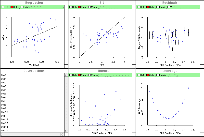
Visualization: ViSta DOES (last year it didn't) produce a visualization for simple regression. Here it is:



See the help files for this visualization.

---