Statistics, Science, and Observations

Statistics, Science, and Observations

Overview

The two most fundamental concepts underlying inferential statistics are introduced in this lecture. These are:

1. Sampling Distributions which are distributions of sample statistics (such as the mean), not of observations.
2. The Central Limit Theorem which allows us to
   • find the probability of getting any specific sample. We discuss this in this lecture.
   • make inferences from samples about populations. We begin discussion of this next week, and continue for the remainder of the semester.

Three types of Distributions

Sample Distribution

A sample distribution is an observed distribution of the values that a variable is observed to have for a sample of individuals. We have seen numerous sample distributions.

Population Distribution

A population distribution is a theoretical distribution of the values that a variable can take on in a population of individuals. We have also learned about population distributions (normal and binomial).

Sampling Distribution

A sampling distribution is a theoretical distribution of the values that a specified statistic of a sample takes on in all of the possible samples of a specific size that can be made from a given population. We have not discussed sampling distributions before.

Note that we can have sampling distributions of sample means, of sample standard deviations, etc.

Demonstration of Sampling Distributions

Example:

SAT Math Sample Distribution

Consider the SAT-Math variable that we observed in the survey done on the first day of class. This example is from 1997. You can download the 1999 data and compare results.

Sample Statistics, Population Parameters and Sample Frequency Distribution for SAT Math
Statistics & Parameters	Sample Frequency Distribution
Sample Statistics Samp. Mean = 589.39 Samp. Stand. Dev. = 94.35	Legend: Red = males; Blue = females.
Population Parameters Pop. Mean = 460 Pop. Stand. Dev. = 100

SAT MATH SAMPLE DISTRIBUTION
Samp. Mean = 589.39
Samp. Stand. Dev. = 94.35

SAT Math Population Distribution

The population distribution for SAT Math scores is a normal distribution with mean of 460 and standard deviation of 100.


SAT Math Population Distribution: Normal, Mean=460, StDv=100

SAT Math Distribution of Sample Means (n=41)

The Distribution of sample means, for samples of size n=41, when the population has a mean of 460 and a standard deviation of 100, is:


SAT Math Sampling Distribution of means
Samples size n=41 (Std.Err.=15.6)
(We'll know what the Std.Err. is by the end of the lecture!)

So What? We can determine how likely it is that the class is a sample that came from the general population of those taking the SAT Math examination.

Your sample mean is 589.39. We will conclude it is very very very very unlikely (probability is within 16 decimal places of 0) to get a sample like this from the general population of those taking the SAT Math exam.

Conclusion: This class is not a sample from the general population of those taking the SAT Math exam! Your average score is much much much much better! (But, we knew that all along :-)

How do we do this? We need to understand Sampling Distributions and the Central Limit Theorem!

Here we go ...

Sampling Distribution of Sample Means

Definition: Sampling Distribution

A sampling distribution is a theoretical distribution of the values that a specified statistic of a sample takes on in all of the possible samples of a specific size that can be made from a given population.

Definition: Distribution of Sample Means (the full name is Sampling Distribution of Sample Means)

A sampling distribution of sample means is a theoretical distribution of the values that the mean of a sample takes on in all of the possible samples of a specific size that can be made from a given population.

Example from Graveter and Wallnau

The point of this example is:

1. Even though the population is not normal, the sampling distribution will approximate a normal distribution.
2. The approximation becomes better as the sample size gets larger.

Graveter and Wallnau consider a population that only has 4 scores:
[2, 4, 6, 8].
This population is very non-normal (it's called "uniform"). It's distribution looks like this:


Population Distribution
for [2, 4, 6, 8]
This Population is very non-normal (uniform)

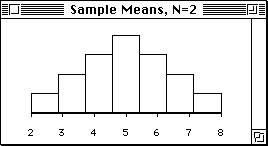
Graveter and Wallnau use this population as the basis for constructing a distribution of sample means for sample size of 2 (that is: N=2). They explain how this distribution is constructed. The distribution is shown below:


Sampling Distribution of Sample Means (N=2)
This distribution is only roughly normal.

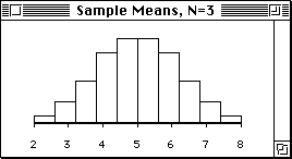
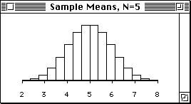
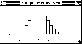
We extend their example by constructing distributions of sample means for sample sizes of N=3, N=4 and N=5, following the same approach taken by Graveter and Wallnau. All four sampling distributions of the sample means are shown below. You can download the ViSta Applet that creates these distributions.


Sampling Distribution of Sample Means (N=3)
Normality is better than those above.


Sampling Distribution of Sample Means (N=4)
Normality is even better than those above.


Sampling Distribution of Sample Means (N=5)
This distribution is very normal.


Sampling Distribution of Sample Means (N=6)
This distribution is even more normal.

To repeat the point of this example:

1. Even though the population is not normal, the sampling distribution will approximate a normal distribution.
2. The approximation becomes better as the sample size gets larger.

The Central Limit Theorem

In the example just given above, we were able to exactly determine the distribution of sample means. We could do this because the population was so simple, having only four scores.

Usually, we can't do this.

When we can't exactly determine the distribution of sample means, we can use the central limit theorem to understand its general characteristics. This is also true for the distribution of other sample statistics.

For this reason, the central limit theorem serves as a cornerstone of much of inferential statistics.

Definition:

The Central Limit Theorem (C.L.T.): For any population with mean and standard deviation
and ,
the distribution of sample means for sample size n will, as n approaches infinity, approach a normal distribution with mean and standard deviation
and .

Demonstration of Central Limit Theorem

The Central Limit Theorem is the most important point of the semester!

WHY? Because of the following two points:

1. The C.L.T. describes the distribution of sample means (or of any other sample statistics) of any population, no matter what shape, mean or standard deviation it has.
2. The distribution of sample means approaches normality very rapidly. By the time the sample reaches n-30, the distribution is almost perfectly normal. Just look at our example!

The C.L.T. describes the distribution of sample means (and any other sampling distribution) according to three characteristics:

1. The SHAPE tends to be normal. It will be almost perfectly normal if
   • The population from which the samples are drawn are normal
   • The sample size (n) in each sample is relatively large, around 30 or more.
2. The MEAN of the distribution of sample means.
   • The expected value is the name given to the mean of the distribution of sample means (or of any other sample statistic).
   • The expected value is equal to the population mean (or other sample statistic).
3. The STANDARD DEVIATION of the distribution of sample means.
   • The standard error is the name given to the standard deviation of the distribution of sample means (or of any other sample statistic).
   • The smaller the population standard deviation, the smaller the standard error.
   • The standard error is equal to the standard deviation of the population divided by the square root of the sample size.
     
   • The larger the sample size, the smaller the standard error.

ViSta C.L.T. Applet

ViSta Applet on Central Limit Theorem. This can be done in ViSta directly by simply using the FILE MENU's SIMULATE DATA menu item.

Probability and the Sampling Distribution

We now know how to calculate the distribution of sample means for SAT Math scores (i.e., the SAT Math sampling distribution of means).

We know that

1. SHAPE: The distribution is normal.
2. MEAN: The mean = 460.
3. STANDARD ERROR: The standard error (standard deviation of the sampling distribution) of sample means is calculated using the following formula
   

   Thus, we can draw the distribution. Here it is:

   
   SAT Math Sampling Distribution of means
   Samples size n=41 (Std.Err.=15.6)

   We can use the distribution of sample means to answer the following question:

   Given that the scores on the SAT Math exam follow a normal distribution with a mean of 460 and a standard deviation of 100, what is the probability of obtaining this class's sample of scores (mean=589.93, N=41)? (We now know that the sampling distribution of sample means is normal with a mean of 460 and a standard error of 15.6).

   We answer this question by calculating the Z-score for the mean of the scores on the SAT Math exam reported by members of this class (the sample).

   This means that the Z-score for your SAT Math sample mean of 589.39 is:
   

   This Z-score is so large it is not in any Z tables. If we use ViSta to calculate the probability of getting such a Z-score it tells us it is 0.00 (which actually means it is less than .0000000000000001).

   Thus, our answer to the question above is that the probability is (essentially) zero that the members of this class represent a sample drawn at random from the general population of those taking the SAT math examination.

   Conclusion: As we said at the outset, this class is not a sample from the general population of those taking the SAT Math exam! Your average score is much much much much better!

---